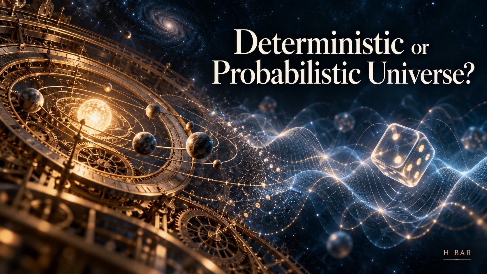

~From Laplace’s demon and chaos to quantum probability and the limits of free will~
A deterministic or probabilistic universe? The question begins with two apparently simple scenes. One billiard ball strikes another and changes its course. If we knew the positions, velocities, masses and forces with absolute precision, we could, at least in principle and within the classical model, calculate where each ball would come to rest. A radioactive atom, by contrast, may decay in the next minute or remain unchanged for years. Quantum mechanics gives us the probability of its decay, rather than the exact moment at which it will occur.
These two pictures seem to describe two different universes. In the first, the future follows necessarily from the present. In the second, nature seems to leave room for genuinely different possibilities. Yet the contrast is not so simple. A deterministic system can be unpredictable, while a probabilistic theory can predict the behaviour of large ensembles with remarkable accuracy. Neither picture, on its own, settles the problem of human freedom.
Newton’s mechanical universe

The great success of classical mechanics encouraged a new metaphysical confidence. Newton’s laws connected the fall of an apple with the motion of the Moon. The same equations could explain planetary orbits, the flight of a projectile and the oscillation of a pendulum. Nature began to resemble a mechanism: complex, but not arbitrary.
In a well-posed classical model, the laws of motion and initial conditions determine how the system evolves. If we know a body’s position and velocity at a particular moment, together with the forces acting on it, the equations allow us to calculate its subsequent state. Determinism does not simply mean that every event has a cause. It means that exactly the same past and the same laws allow only one possible future.
Pierre-Simon Laplace expressed this idea especially clearly. In 1814, he imagined an intelligence that knew all the forces and all the positions of matter. If it could analyse those data, nothing would be uncertain: the past and future would be equally clear to it. Laplace himself did not call this intelligence a “demon”; that name came later. The image nevertheless endured as the emblem of complete scientific determinism. 1
Determinism does not mean predictability

Laplace’s demon required two things: perfect knowledge of the present and unlimited computational power. A real observer has neither. Chaos theory made the consequences of that difference dramatically clear.
In 1963, meteorologist Edward Lorenz studied a simple system of three differential equations representing idealised atmospheric convection. The equations were entirely deterministic. Yet two initial states that differed only slightly could diverge greatly over time. The evolution still obeyed the laws, while long-range prediction became unreliable. 2
This is sensitive dependence on initial conditions. Every measurement has finite precision. If a tiny initial error grows exponentially, then beyond a certain time two almost identical descriptions can produce radically different predictions. Weather is the best-known example, but chaotic behaviour also occurs in fluids, ecosystems, electrical circuits and celestial systems.
Chaos does not necessarily introduce randomness into the laws. It exposes a limit to our knowledge. A system can be ontologically deterministic, with a unique evolution, and still be epistemically unpredictable for a finite observer. The distinction matters: what nature determines is not the same as what we can calculate.
Probability before quantum mechanics
Probability did not have to wait for quantum physics to enter science. A gas contains an enormous number of molecules whose motion can be modelled using classical laws. Nobody tracks every trajectory individually. Statistical mechanics describes distributions of velocities, pressure, temperature and entropy. Uncertainty about microscopic states becomes a framework for precise predictions of macroscopic behaviour. 3
Here, probability can be epistemic: it need not mean that molecules “decide” at random, only that we do not possess, or do not need, every detail. We toss a coin and speak of probability because we do not know its exact initial conditions, rotation, air resistance and collisions. The outcome can be practically unpredictable without being fundamentally indeterminate.
Statistical mechanics also reveals something deeper. Although many microscopic mechanical laws are time-reversal invariant, heat disperses and macroscopic entropy typically increases from suitable low-entropy initial conditions. This arrow of time is a statistical regularity, not something that follows from reversible laws alone. Probability is more than an admission of ignorance: it is a language through which new regularities emerge at another level of description.
The quantum turning point

Quantum mechanics changed the question. Between measurements, the wavefunction evolves smoothly and deterministically according to the Schrödinger equation. But when a measurement is performed, the usual quantum rules do not generally assign one certain outcome. They assign probabilities to the different possible outcomes. Whether this means that nature itself is fundamentally indeterministic depends on how the theory is interpreted.
Imagine that we want to measure an electron’s position. Its wavefunction, denoted by ψ, does not, by itself, identify one point at which the electron must be found. It is more like a map of possible detection locations: some regions are more likely than others.
Born’s rule is the mathematical prescription that converts this “map of possibilities” into probabilities. For a normalised pure state and a non-degenerate measurement outcome associated with the normalised eigenstate labelled aᵢ, it reads:
The quantity inside the modulus is called a probability amplitude. It is not yet a probability: it may be negative or complex. A probability must be a real number between zero and one, so we take the squared modulus of the amplitude. For example, if an outcome’s amplitude has modulus 0.5, its probability is 0.5² = 0.25, or 25%.
For a particle’s position in one dimension, we write:
Here, ρ is a probability density, rather than the probability of an exact position. The probability of finding the particle within a region is obtained by integrating the density over that region. Integrating over all possible positions gives one: a total probability of 100%. 4
Suppose Born’s rule gives a 25% probability that an electron will appear in a particular region of a screen. This does not mean that every fourth electron must arrive there in a fixed sequence. It means that, over many repetitions with the same preparation, the relative frequency will tend towards one quarter. We cannot generally predict the next individual detection, but we can predict the overall distribution with great accuracy.
This is the central feature of quantum probability: the theory may not predict the next individual event, yet it predicts the pattern formed by many events extremely well. The probabilistic prediction is not simply a consequence of a carelessly performed experiment. It remains even when the state preparation is controlled as fully as the theory permits.
What did Bell set out to test?
In its usual measurement formulation, quantum mechanics gives us probabilities rather than a hidden certainty about every individual result. Einstein found it difficult to accept that this uncertainty might be fundamental. He suspected that quantum mechanics could be an incomplete description. Perhaps particles possessed properties unknown to us, the so-called hidden variables, that would account for the outcomes. Apparent randomness might then reflect our ignorance, as it does when we cannot follow a coin’s motion precisely.
In 1964, John Bell showed that an important class of such proposals could be tested experimentally. Could quantum correlations be explained by local hidden properties, while the measurement settings were chosen independently of those properties? 5
“Local” means more than an inability to send a usable instantaneous message. In a locally causal model, a sufficiently complete account of relevant common causes makes each side’s outcome independent of the distant setting and outcome. The independence of measurement settings from the hidden variables is a separate assumption. Both matter when interpreting the result.
How is a Bell test organised?

A source creates two entangled particles and sends one to Alice and the other to Bob, who are far apart.
Alice can measure her particle using either of two settings, labelled a and a′. Bob also has two choices, labelled b and b′. These can represent different spin-measurement directions or different angles of photon-polarisation analysis.
In the idealised binary-outcome version of the test:
- Alice randomly selects one of her two settings.
- Bob independently selects one of his.
- Each measurement returns one of two outcomes, labelled +1 and −1.
The signs do not denote positive and negative electric charge. They simply label the two possible readings: for example, detection in one output channel or the other.
The experiment is repeated many times. Alice and Bob examine not only the individual results but also how often their outcomes agree or disagree for each combination of settings. In the idealised case, the correlation is estimated by:
If the outcomes always agree, the correlation is +1. If they always disagree, it is −1. An unbiased pair of uncorrelated outcome streams gives a value close to zero.
For actual photon experiments, missed detections must also be handled correctly. The 2015 photon tests used Bell inequalities and statistical procedures designed to avoid relying on a selectively retained sample of coincident detections. The simple correlation formula above explains the idea; it is not a complete data-analysis recipe for every experiment. 6, 8, 9
Why does the bound of two appear?
The four combinations of measurement settings enter the CHSH quantity:
Imagine, as a simple model, that each particle carries predetermined responses for all the possible local settings. If those responses are local and the settings are statistically independent of the hidden variables, the correlations cannot take arbitrary values. They obey:
This limit is a mathematical consequence of the model’s assumptions, not a peculiarity of the detectors. More generally, it also holds for locally causal stochastic hidden-variable models satisfying measurement independence; the result does not exclude only deterministic “instruction sheets”. 5, 6
Quantum mechanics predicts a different bound. With suitable states and measurement directions, it permits:
Thus, a statistically reliable violation of the local bound cannot be explained by that class of local models while retaining the assumptions used to derive it.
This does not mean that Alice can send Bob a message faster than light. Quantum correlations do not provide controllable faster-than-light signalling. The correlation pattern is established when the two sides later compare their records.
Closing the experimental loopholes
Early Bell tests agreed with quantum mechanics but left experimental loopholes. If the stations were too close, or measurements took too long, an ordinary signal could potentially pass between them during the relevant events.
Older detectors also registered only a fraction of the particles. A local model could exploit this if the detected events formed an unrepresentative sample.
The settings therefore needed to be selected rapidly and with carefully controlled spacetime relationships. This restricts possible connections between the source, the settings and the distant measurement. It does not establish independence from every conceivable hidden common cause without further assumptions.
In 2015, three independent teams performed tests designed to close the major detection and locality loopholes simultaneously, while carefully addressing the generation of measurement settings. 7, 8, 9
The Delft experiment: two spins 1.3 kilometres apart
In Delft, in the Netherlands, the researchers used tiny defects in diamonds known as nitrogen-vacancy centres. At each centre they could control and measure an electron’s spin.
The diamonds were located in laboratories 1.3 kilometres apart. Each side emitted a photon entangled with its local electron spin. The photons met at an intermediate station, where particular detection events heralded entanglement between the distant spins.
After this confirmation, Alice and Bob randomly selected their spin-measurement settings. The choices and measurements were completed quickly enough to maintain the required spacelike separation.
The experiment’s advantage was highly efficient spin readout. Its limitation was that successful remote entanglement generation was rare: only 245 valid trials were collected. Even so, the data violated the local bound. The reported CHSH value was 2.42 ± 0.20. 7

The photon experiments in Vienna and at NIST
The Vienna and NIST teams used a different approach. Laser pulses drove a crystal source that produced pairs of polarisation-entangled photons.
One photon travelled towards Alice and the other towards Bob. While the photons were in flight, fast random-number generators selected the polarisation-analysis settings. The measurement apparatus therefore did not use one fixed, prearranged sequence of settings.
Highly efficient superconducting detectors helped close the detection loophole. The technologies differed: Vienna used transition-edge sensors, while NIST used superconducting nanowire detectors. The two NIST stations were 184 metres apart; the Vienna stations were about 58 metres apart. In each experiment, the timing and separation were designed so that the relevant choices and measurements were spacelike separated. 8, 9
Despite their different technologies, the experiments supported the same central conclusion: the observed correlations violated the relevant locally causal models under the stated assumptions.
What did the experiments establish?
Bell tests did not prove that “everything happens randomly”. They did not show that we can communicate instantaneously, or that quantum mechanics has only one possible philosophical interpretation.
They did rule out a particularly attractive picture under explicit conditions: particles carrying only local hidden instructions, independent of the later choices of measurement settings, cannot reproduce the observed correlations.
The broader lesson is that local causality, measurement independence and the observed quantum correlations cannot all be retained together in a model satisfying the Bell assumptions. Abandoning determinism alone is not enough to evade this result. Nonlocal deterministic accounts remain possible, while proposals that reject measurement independence require a different discussion of the assumptions. 5, 6
One theory, many accounts of reality

Quantum mechanics is extraordinarily successful as a predictive framework, but its interpretation remains contested. In many Copenhagen-style accounts, measurement outcomes are treated as fundamentally probabilistic. De Broglie–Bohm theory, by contrast, is deterministic: particles have definite positions and are guided by the wavefunction, at the price of an explicitly nonlocal structure. 10
In Everett’s relative-state approach and its many-worlds developments, the universal wavefunction never collapses. Its overall evolution is deterministic, while different measurement records occur in different branches. Probability must then be understood through branch weights and the observer’s relation to future experiences. Exactly how to justify the usual probability rule in this framework remains a matter of debate. 11
Objective-collapse theories take another route. They change the dynamics so that collapse becomes an actual stochastic physical process. These are testable modifications of quantum mechanics, not merely alternative verbal interpretations of exactly the same equations; they can predict departures from standard theory. 12
These approaches agree on many successful quantum predictions while differing over what exists and, in some cases, over predictions in regimes where their dynamics diverge. The evidence does not turn a successful probabilistic prediction into one final metaphysical conclusion. Physics has sharply constrained the easy answers without settling every possible account of reality.
The universe as an initial condition
Even if the laws were fully deterministic, the question of initial conditions would remain. Why did the universe begin in this state rather than another? Laws describe how a state evolves; they do not always explain why that particular state obtained.
In contemporary cosmology, small primordial perturbations provide the seeds from which galaxies and large-scale structure formed. Inflationary models commonly describe their origin in terms of quantum fluctuations. Observations constrain their statistical properties, but do not by themselves establish one unique inflationary model or a final interpretation of quantum probability. A probabilistic model can predict a spectrum of perturbations without giving one uniquely determined story for every galaxy. 13
The opposition between “law” and “chance” may therefore be too narrow. The actual universe may combine stable laws, particular initial conditions, chaotic amplification of small differences and quantum probabilities. Order and contingency need not be opponents. They can operate at different levels of the same description.
Randomness is not freedom
The question becomes personal when it reaches free will. If every state of the brain follows necessarily from the previous one, were our decisions unavoidable before we were born? If some neural processes are affected by quantum randomness, does that make us freer?
The second suggestion is less straightforward than it sounds. A random event in the brain is not, simply by being random, an exercise of agency. Replacing necessity with a quantum die does not by itself create responsibility, intention or control. Quantum probability does not supply evidence that consciousness can direct measurement outcomes at will. 14
Compatibilism offers another route. Freedom, in this view, need not mean an absence of causes. It can involve the ability to act in response to reasons, values and desires without coercion. The fact that decisions have causes does not automatically make them alien to us: those causes include character, memory, reflection and responsiveness to arguments. Incompatibilists object that this may not be enough, since character itself has a history we did not choose. The disagreement is not settled by a physics experiment alone; it also concerns what we mean by saying, “I could have acted otherwise.” 14, 15
A universe more complex than the dilemma
Do we inhabit a deterministic or probabilistic universe? The most honest answer is that physics has not selected one final metaphysical picture. But we know enough to reject the simplest versions of the dilemma.
Classical mechanics demonstrated the power of deterministic laws. Chaos showed that determinism does not guarantee predictability. Statistical mechanics showed how probabilities can support robust macroscopic regularities. Quantum mechanics placed probability at the heart of our best physical predictions, while Bell tests ruled out a broad class of local explanations under explicit assumptions. Different interpretations nevertheless remind us that the mathematical formalism and our account of the world are not exactly the same thing.
Perhaps the most important lesson is not whether the future is already written or is written as it happens. It is that reality resists both easy metaphors. It is neither merely a clock nor merely a die. It is a web of laws, possibilities and limits to knowledge, within which human freedom remains not a gap between causes, but a question about what it means to be the agents of our actions.
Sources and further reading
- Laplace, P.-S. (1814; English translation 1902). A Philosophical Essay on Probabilities, Chapter II.
- Lorenz, E. N. (1963). Deterministic Nonperiodic Flow. Journal of the Atmospheric Sciences 20, 130–141.
- Gibbs, J. W. (1902). Elementary Principles in Statistical Mechanics.
- MIT OpenCourseWare (2013). 8.04 Quantum Physics I, Problem Set 2 Solutions, Problem 3: Born interpretation and probability density.
- Bell, J. S. (1964). On the Einstein Podolsky Rosen paradox. Physics Physique Fizika 1, 195–200.
- Clauser, J. F., Horne, M. A., Shimony, A. & Holt, R. A. (1969). Proposed Experiment to Test Local Hidden-Variable Theories. Physical Review Letters 23, 880–884.
- Hensen, B. et al. (2015). Loophole-free Bell inequality violation using electron spins separated by 1.3 kilometres. Nature 526, 682–686.
- Giustina, M. et al. (2015). Significant-Loophole-Free Test of Bell’s Theorem with Entangled Photons. Physical Review Letters 115, 250401. Open manuscript included.
- Shalm, L. K. et al. (2015). Strong Loophole-Free Test of Local Realism. Physical Review Letters 115, 250402. NIST publication record.
- Bohm, D. (1952). A Suggested Interpretation of the Quantum Theory in Terms of Hidden Variables. I. Physical Review 85, 166–179.
- Everett, H. III (1957). “Relative State” Formulation of Quantum Mechanics. Reviews of Modern Physics 29, 454–462.
- Bassi, A., Lochan, K., Satin, S., Singh, T. P. & Ulbricht, H. (2013). Models of wave-function collapse, underlying theories, and experimental tests. Reviews of Modern Physics 85, 471–527.
- Planck Collaboration (2020). Planck 2018 results. X. Constraints on inflation. Astronomy & Astrophysics 641, A10.
- Stanford Encyclopedia of Philosophy. Free Will.
- Stanford Encyclopedia of Philosophy. Compatibilism.
Change is the only Constant